41 show data labels excel

Find, label and highlight a certain data point in Excel ... Select the Data Labels box and choose where to position the label. By default, Excel shows one numeric value for the label, y value in our case. To display both x and y values, right-click the label, click Format Data Labels…, select the X Value and Y value boxes, and set the Separator of your choosing: Label the data point by name Custom Chart Data Labels In Excel With Formulas Follow the steps below to create the custom data labels. Select the chart label you want to change. In the formula-bar hit = (equals), select the cell reference containing your chart label's data. In this case, the first label is in cell E2. Finally, repeat for all your chart laebls.

How to format axis labels as thousands/millions in Excel? 3. Close dialog, now you can see the axis labels are formatted as thousands or millions. Tip: If you just want to format the axis labels as thousands or only millions, you can type #,"K" or #,"M" into Format Code textbox and add it.

Show data labels excel

How to add data labels from different column in an Excel ... Right click the data series, and select Format Data Labels from the context menu. 3. In the Format Data Labels pane, under Label Options tab, check the Value From Cells option, select the specified column in the popping out dialog, and click the OK button. Now the cell values are added before original data labels in bulk. 4. How to Add Labels to Scatterplot Points in Excel - Statology Step 3: Add Labels to Points Next, click anywhere on the chart until a green plus (+) sign appears in the top right corner. Then click Data Labels, then click More Options… In the Format Data Labels window that appears on the right of the screen, uncheck the box next to Y Value and check the box next to Value From Cells. How to hide zero data labels in chart in Excel? If you want to hide zero data labels in chart, please do as follow: 1. Right click at one of the data labels, and select Format Data Labels from the context menu. See screenshot: 2. In the Format Data Labels dialog, Click Number in left pane, then select Custom from the Category list box, and type #"" into the Format Code text box, and click Add button to add it to Type list box.

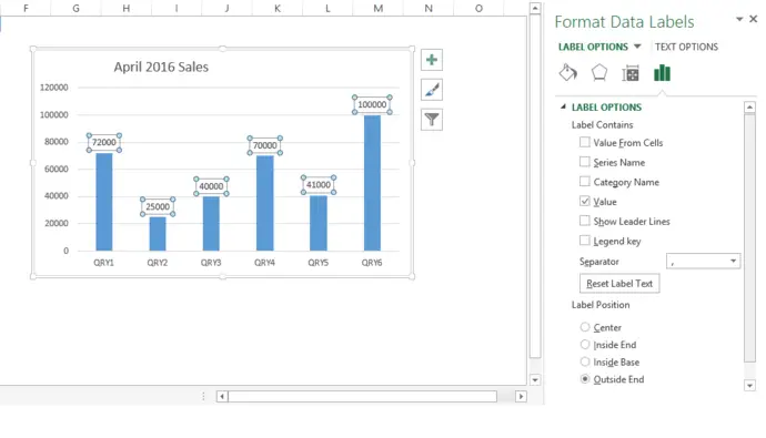
Show data labels excel. Edit titles or data labels in a chart The first click selects the data labels for the whole data series, and the second click selects the individual data label. Right-click the data label, and then click Format Data Label or Format Data Labels. Click Label Options if it's not selected, and then select the Reset Label Text check box. Top of Page How to add or move data labels in Excel chart? In Excel 2013 or 2016. 1. Click the chart to show the Chart Elements button . 2. Then click the Chart Elements, and check Data Labels, then you can click the arrow to choose an option about the data labels in the sub menu. See screenshot: In Excel 2010 or 2007. 1. click on the chart to show the Layout tab in the Chart Tools group. See ... Excel charts: how to move data labels to legend ... @Matt_Fischer-Daly . You can't do that, but you can show a data table below the chart instead of data labels: Click anywhere on the chart. On the Design tab of the ribbon (under Chart Tools), in the Chart Layouts group, click Add Chart Element > Data Table > With Legend Keys (or No Legend Keys if you prefer) Can you display data labels on a trend line? | MrExcel ... Hi I have plotted some sales figures on a line chart (Jan-Aug), and added a linear trend line to view the trend to the end of the year. I have not used the 'forecast forward 4 periods' feature to do this, instead I have just selected an additional 4 blank rows below the 'august' line - which extends the x axis, and therefore extends the trend line.

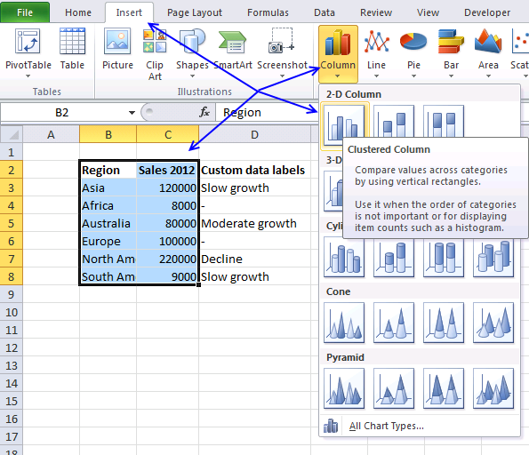
Move data labels - support.microsoft.com Right-click the selection > Chart Elements > Data Labels arrow, and select the placement option you want. Different options are available for different chart types. For example, you can place data labels outside of the data points in a pie chart but not in a column chart. Series.DataLabels method (Excel) | Microsoft Docs Data labels can be turned on or off for individual points in the series. If the series is on an area chart and has the Show Label option turned on for the data labels, the returned collection contains only a single label, which is the label for the area series. Example. This example sets the data labels for series one on Chart1 to show their ... How to Customize Your Excel Pivot Chart Data Labels - dummies The Data Labels command on the Design tab's Add Chart Element menu in Excel allows you to label data markers with values from your pivot table. When you click the command button, Excel displays a menu with commands corresponding to locations for the data labels: None, Center, Left, Right, Above, and Below. None signifies that no data labels should be added to the chart and Show signifies ... How to Change Excel Chart Data Labels to Custom Values? First add data labels to the chart (Layout Ribbon > Data Labels) Define the new data label values in a bunch of cells, like this: Now, click on any data label. This will select "all" data labels. Now click once again. At this point excel will select only one data label. Go to Formula bar, press = and point to the cell where the data label ...

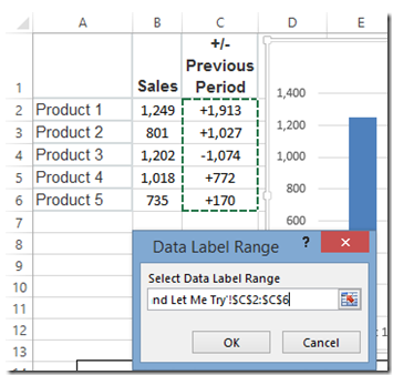
Add or remove data labels in a chart Right-click the data series or data label to display more data for, and then click Format Data Labels. Click Label Options and under Label Contains, select the Values From Cells checkbox. When the Data Label Range dialog box appears, go back to the spreadsheet and select the range for which you want the cell values to display as data labels. Change the format of data labels in a chart To get there, after adding your data labels, select the data label to format, and then click Chart Elements > Data Labels > More Options. To go to the appropriate area, click one of the four icons ( Fill & Line, Effects, Size & Properties ( Layout & Properties in Outlook or Word), or Label Options) shown here. Chart.ApplyDataLabels method (Excel) | Microsoft Docs For the Chart and Series objects, True if the series has leader lines. Pass a Boolean value to enable or disable the series name for the data label. Pass a Boolean value to enable or disable the category name for the data label. Pass a Boolean value to enable or disable the value for the data label. Add a DATA LABEL to ONE POINT on a ... - Excel Quick Help Steps shown in the video above: Click on the chart line to add the data point to. All the data points will be highlighted. Click again on the single point that you want to add a data label to. Right-click and select ' Add data label ' This is the key step! Right-click again on the data point itself (not the label) and select ' Format data label '.

Format Number Options for Chart Data Labels in Excel 2011 for Mac

How to create a chart with both percentage and value in Excel? After installing Kutools for Excel, please do as this:. 1.Click Kutools > Charts > Category Comparison > Stacked Chart with Percentage, see screenshot:. 2.In the Stacked column chart with percentage dialog box, specify the data range, axis labels and legend series from the original data range separately, see screenshot:. 3.Then click OK button, and a prompt message is popped out to remind you ...

Parts of a Spreadsheets

Excel tutorial: How to use data labels Generally, the easiest way to show data labels to use the chart elements menu. When you check the box, you'll see data labels appear in the chart. If you have more than one data series, you can select a series first, then turn on data labels for that series only. You can even select a single bar, and show just one data label.

Pie Chart - PK: An Excel Expert

Solved: why are some data labels not showing? - Microsoft ... Please use other data to create the same visualization, turn on the data labels as the link given by @Sean. After that, please check if all data labels show. If it is, your visualization will work fine. If you have other problem, please let me know. Best Regards, Angelia. Message 3 of 4.

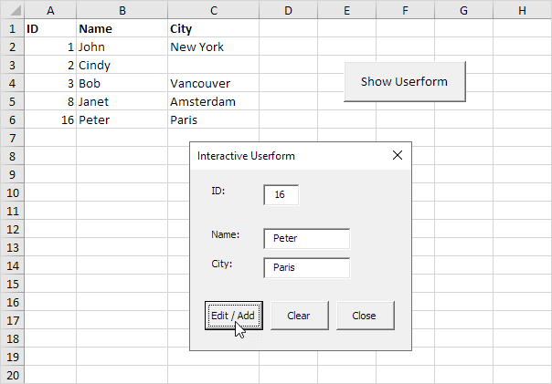
Excel VBA Interactive Userform - Easy Excel Macros

Format Data Labels in Excel- Instructions - TeachUcomp, Inc. To do this, click the "Format" tab within the "Chart Tools" contextual tab in the Ribbon. Then select the data labels to format from the "Chart Elements" drop-down in the "Current Selection" button group. Then click the "Format Selection" button that appears below the drop-down menu in the same area.

How to Print Labels from Excel

DataLabels.ShowValue property (Excel) | Microsoft Docs Example. This example enables the value to be shown for the data labels of the first series, on the first chart. This example assumes that a chart exists on the active worksheet. VB. Sub UseValue () ActiveSheet.ChartObjects (1).Activate ActiveChart.SeriesCollection (1) _ .DataLabels.ShowValue = True End Sub.

Download Kutools for Excel 23.00

How to show data label in "percentage" instead of ... Select Format Data Labels Select Number in the left column Select Percentage in the popup options In the Format code field set the number of decimal places required and click Add. (Or if the table data in in percentage format then you can select Link to source.) Click OK Regards, OssieMac Report abuse 8 people found this reply helpful ·

Formula Friday - Using Formulas To Add Custom Data Labels To Your Excel Chart - How To Excel At ...

Excel tutorial: Dynamic min and max data labels To show you how this works, I'll first add a column next the data, and manually flag the minimum and maximum values. Now, back in the label options area, I'll uncheck Value, and check "Value from cells". Then I need to select the new column. When I click OK, the existing data labels are replaced by the labels I typed by hand. So that's the concept.

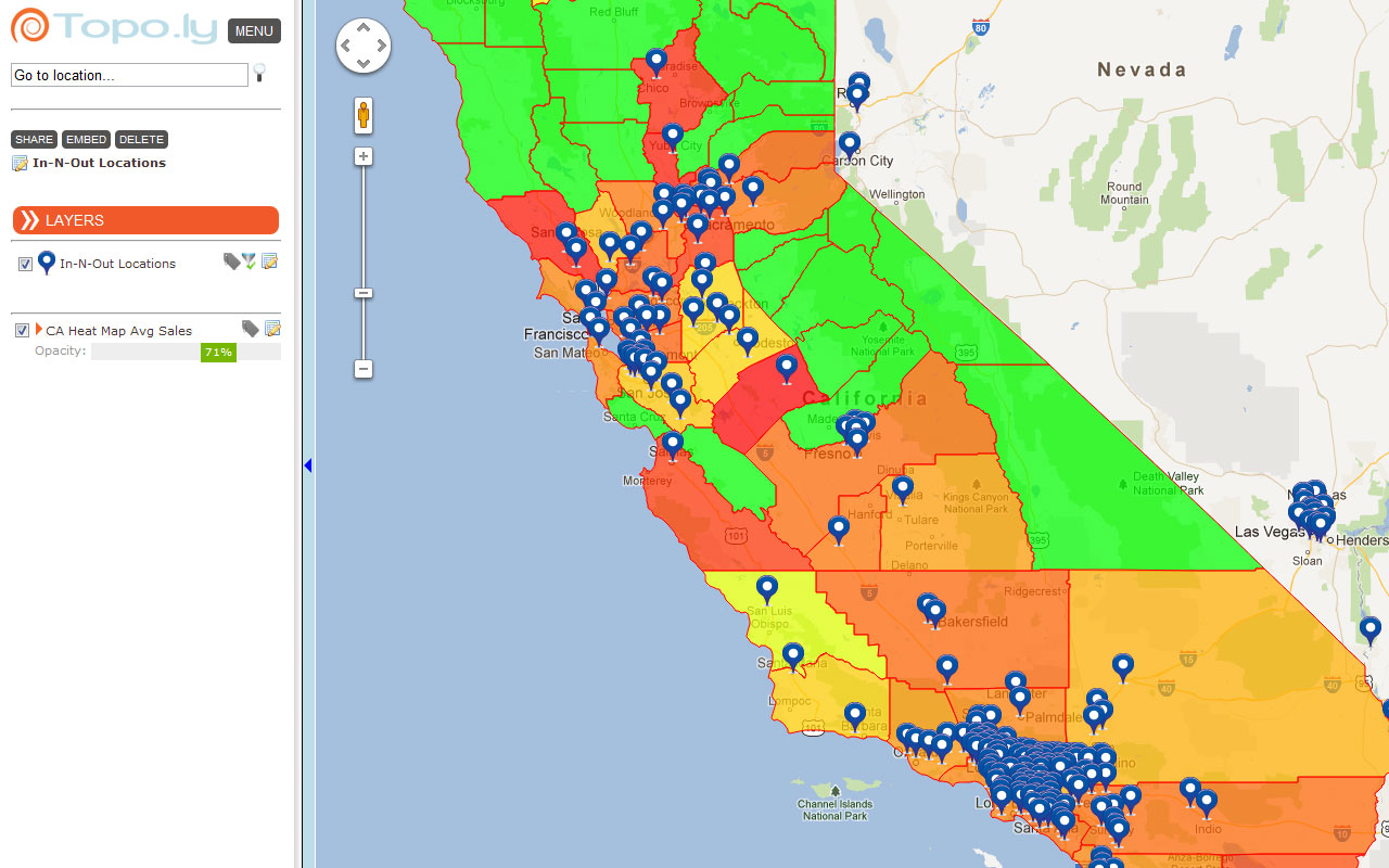
Improve Data Visualization By Mapping with Microsoft Excel | Pressat

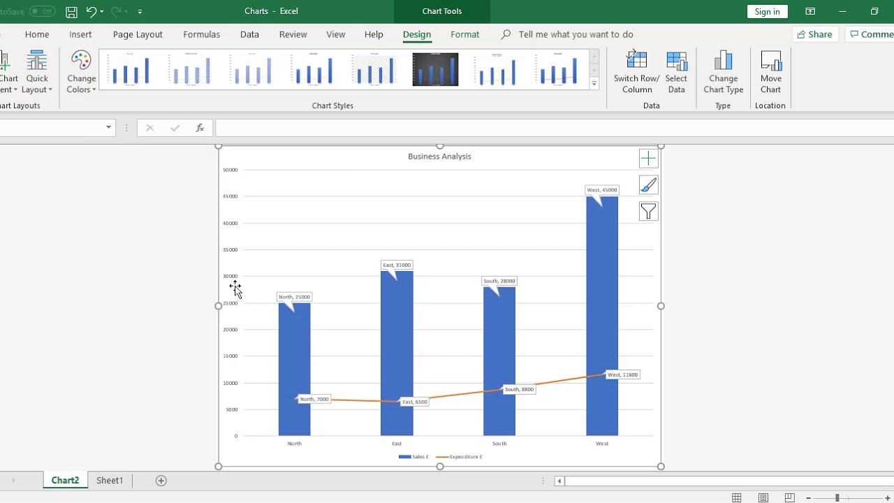
Show or hide a chart legend or data table To show a data table, point to Data Table and select the arrow next to it, and then select a display option. To hide the data table, uncheck the Data Table option. Show or hide a legend. Click the chart in which you want to show or hide a legend. This displays the Chart Tools, adding the Design, Layout, and Format tabs.

Display Excel data table nicely on mobile phones, without coding | by Leroy Yue | PikaPage | Medium

Excel 2010: Show Data Labels In Chart - AddictiveTips With data labels, you can easily view the values that affects chart area in Excel 2010. Lets look at how to enable and use them. To enable data labels in chart, select the chart and head over to Chart Tools Layout tab, from Labels group, under Data Labels options, select a position. It will show Data labels at specified position.

30 What Is A Data Label In Excel - Labels Database 2020

How to hide zero data labels in chart in Excel? If you want to hide zero data labels in chart, please do as follow: 1. Right click at one of the data labels, and select Format Data Labels from the context menu. See screenshot: 2. In the Format Data Labels dialog, Click Number in left pane, then select Custom from the Category list box, and type #"" into the Format Code text box, and click Add button to add it to Type list box.

How to Add Data Labels to your Excel Chart in Excel 2013 - YouTube

How to Add Labels to Scatterplot Points in Excel - Statology Step 3: Add Labels to Points Next, click anywhere on the chart until a green plus (+) sign appears in the top right corner. Then click Data Labels, then click More Options… In the Format Data Labels window that appears on the right of the screen, uncheck the box next to Y Value and check the box next to Value From Cells.