38 excel chart only show certain data labels

Excel tutorial: How to use data labels In this video, we'll cover the basics of data labels. Data labels are used to display source data in a chart directly. They normally come from the source data, but they can include other values as well, as we'll see in in a moment. Generally, the easiest way to show data labels to use the chart elements menu. When you check the box, you'll see ... Create a chart from start to finish However, the chart data is entered and saved in an Excel worksheet. If you insert a chart in Word or PowerPoint, a new sheet is opened in Excel. When you save a Word document or PowerPoint presentation that contains a chart, the chart's underlying Excel data is automatically saved within the Word document or PowerPoint presentation.

Excel charts: add title, customize chart axis, legend and data labels Click anywhere within your Excel chart, then click the Chart Elements button and check the Axis Titles box. If you want to display the title only for one axis, either horizontal or vertical, click the arrow next to Axis Titles and clear one of the boxes: Click the axis title box on the chart, and type the text.

Excel chart only show certain data labels

How to Insert A Vertical Marker Line in Excel Line Chart Since I have used the Excel Tables, I get structured data to use in the formula.This formula will enter 1 in the cell of the supporting column when it finds the max value in the Sales column. 2: Select the table and insert a Combo Chart: Select the entire table, including the supporting column and insert a combo chart. Goto--> Insert-->Recommended Charts. How to Use Cell Values for Excel Chart Labels - How-To Geek Select the chart, choose the "Chart Elements" option, click the "Data Labels" arrow, and then "More Options.". Uncheck the "Value" box and check the "Value From Cells" box. Select cells C2:C6 to use for the data label range and then click the "OK" button. The values from these cells are now used for the chart data labels. Only Display Some Labels On Pie Chart - Excel Help Forum Only Display Some Labels On Pie Chart. I have a pie chart that contains over 50 categories (Yes, I know pie charts shouldn't be used for that many things) but I want to only display labels for maybe the top 5 values or any label with a value >10. This is because there are a few standout values but I want all the other values to remain in the ...

Excel chart only show certain data labels. How to Only Show Selected Data Points in an Excel Chart Download Free Sample Dashboard Files here: on how to show or hide specific data points i... Suddenly can't select all data labels in a chart at the same time Answer. After selecting all data labels if you then click on one of the selected labels then only that label remains selected. From then on if you click any other label then only the clicked label is selected. To go back to selecting all data labels, click somewhere in the blank part of the plot area which should un-select the selected label. How to create Custom Data Labels in Excel Charts - Efficiency 365 Add default data labels. Click on each unwanted label (using slow double click) and delete it. Select each item where you want the custom label one at a time. Press F2 to move focus to the Formula editing box. Type the equal to sign. Now click on the cell which contains the appropriate label. Press ENTER. Is there a way to show only specific values in x-axis of an excel chart ... 1 Answer. 1) Use a line chart, which treats the horizontal axis as categories (rather than quantities). 2) Use an XY/Scatter plot, with the default horizontal axis "turned off" and replaced with a "helper" series with vertical values of 0 and horizontal values as desired in your dataset (this is my preferred method).

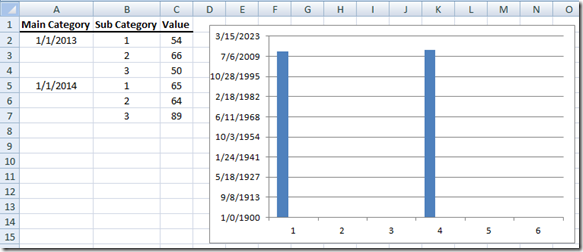
charts - Excel, giving data labels to only the top/bottom X% values ... Here is what you can do, in stages: 1) Create a data set next to your original series column with only the values you want labels for (again, this can be formula driven to only select the top / bottom n values). See column D below. 2) Add this data series to the chart and show the data labels. 3) Set the line color to No Line, so that it does ... Only Show Data Labels in Chart if Value Less than Re: Only Show Data Labels in Chart if Value Less than #. Hi, The simplest way is to create a second data series that excludes the values you don't want to show labels for (eg =IF (A1>=0.2,A1,""). Plot this series with no line or marker, but with the labels showing. Rule 1: Never merge cells. Creating a chart in Excel that ignores #N/A or blank cells I am attempting to create a chart with a dynamic data series. Each series in the chart comes from an absolute range, but only a certain amount of that range may have data, and the rest will be #N/A.. The problem is that the chart sticks all of the #N/A cells in as values instead of ignoring them. I have worked around it by using named dynamic ranges (i.e. Insert > Name > Define), but that is ... Label Specific Excel Chart Axis Dates - My Online Training Hub Steps to Label Specific Excel Chart Axis Dates. The trick here is to use labels for the horizontal date axis. We want these labels to sit below the zero position in the chart and we do this by adding a series to the chart with a value of zero for each date, as you can see below: Note: if your chart has negative values then set the 'Date Label ...

Broken Y Axis in an Excel Chart - Peltier Tech Nov 18, 2011 · You’ve explained the missing data in the text. No need to dwell on it in the chart. The gap in the data or axis labels indicate that there is missing data. An actual break in the axis does so as well, but if this is used to remove the gap between the 2009 and 2011 data, you risk having people misinterpret the data. How to make a chart (graph) in Excel and save it as template 22.10.2015 · 3. Inset the chart in Excel worksheet. To add the graph on the current sheet, go to the Insert tab > Charts group, and click on a chart type you would like to create.. In Excel 2013 and Excel 2016, you can click the Recommended Charts button to view a gallery of pre-configured graphs that best match the selected data.. In this example, we are creating a 3-D Column chart. How to Create a Waterfall Chart in Excel and PowerPoint Mar 04, 2016 · To format the labels, select one of the labels, right-click, and select Format Data Labels from the list. Once the Format Data Labels pane opens, you can adjust the label position, text color and font to make the numbers more readable. *Once you’re done labeling the columns, you can delete unnecessary elements like zero values and the legend. Data Labels - I Only Want One - Google Groups Using X-Y Scatter Plot charts in Excel 2007, I am having trouble getting just one data label to appear for a data series. After selecting just one data point, I right click and select Add Data Label. I am then provided with the Y-value, though I am looking to display the X-value. After right clicking on

Excel Bar Charts - Clustered, Stacked - Template - Automate Excel

How to Make Charts and Graphs in Excel | Smartsheet 22.1.2018 · To Add Up/Down Bars: Up/Down Bars are not available for a column chart, but you can use them in a line chart to show increases and decreases among data points. Step 4: Adjust Quick Layout The second dropdown menu on the toolbar is Quick Layout , which allows you to quickly change the layout of elements in your chart (titles, legend, clusters etc.).

34 How To Label Specific Points In Excel - Labels For You

Highlight a Specific Data Label in an Excel Chart - Peltier Tech Add data labels to each line chart* (left), then format them as desired (right). * right click on the series, choose Add Data Labels from the pop up menu. Finally format the two line chart series so they use no line and no marker. When the data change, the chart labels change just as quickly as Excel can calculate the new values in columns C and D.

Excel tutorial: Dynamic min and max data labels To make the formula easy to read and enter, I'll name the sales numbers "amounts". The formula I need is: =IF (C5=MAX (amounts), C5,"") When I copy this formula down the column, only the maximum value is returned. And back in the chart, we now have a data label that shows maximum value. Now I need to extend the formula to handle the minimum value.

Solved: Show data label only to one line - Power BI On one graph remove all of the lines you don't want to display the data and turn data labels on for this graph. On the second graph remove all of the lines you do want with data. If you then overlay them then you'll have the desigered effect.

Subtotals: Pivot Table/Chart | Formulas | Jan's Working with Numbers

Change the format of data labels in a chart - support.microsoft.com Tip: To switch from custom text back to the pre-built data labels, click Reset Label Text under Label Options. To format data labels, select your chart, and then in the Chart Design tab, click Add Chart Element > Data Labels > More Data Label Options. Click Label Options and under Label Contains, pick the options you want.

Fixing Your Excel Chart When the Multi-Level Category Label Option is Missing. - Excel Dashboard ...

Hiding data labels for some, not all values in a series Here's a good challenge for you. I can't figure it out, and I believe it's a limitation of Excel. I have a bar graph with several data series. I know how to show the data labels for every data point in a given series. But I'm looking to show the data label for only some data points in a given series -- i.e. non-zero valued data points.

How-to Use Data Labels from a Range in an Excel Chart - Excel Dashboard Templates

Chart: only show legend elements with values - MrExcel Message Board However, each graph only needs 3-4 elements out of the 20 legend entries in the graph. Thanks in advance! Not sure how your data is arrange/organised, but you could filter data to show only 'Greater than or equal to' 0 (zero), such would hide the rows with NA () and would display a chart with only data with value.

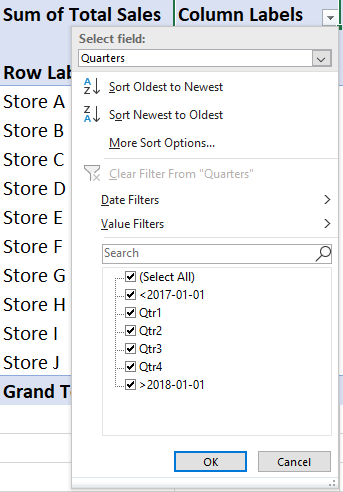
How to Add Filter to Pivot Table: 7 Steps (with Pictures)

How to add data labels from different column in an Excel chart? Please do as follows: 1. Right click the data series in the chart, and select Add Data Labels > Add Data Labels from the context menu to add data labels. 2. Right click the data series, and select Format Data Labels from the context menu. 3.

How to Make Charts and Graphs in Excel | Smartsheet

Prevent Overlapping Data Labels in Excel Charts - Peltier Tech May 24, 2021 · Overlapping Data Labels. Data labels are terribly tedious to apply to slope charts, since these labels have to be positioned to the left of the first point and to the right of the last point of each series. This means the labels have to be tediously selected one by one, even to apply “standard” alignments.

Microsoft Tips with Temo!: How to Add Data Labels to an Excel 2010 Chart

Excel Chart not showing SOME X-axis labels - Super User Apr 05, 2017 · I was having a similar problem and it was only due to what excel can fit in the chart. Click the chart, and then drag one of the sizing handles to enlarge the chart. By default, the fonts in the chart scale proportionally as you resize the chart. Once you make your chart big enough, your labels should show.

Chart-me XLS 2.1

Find, label and highlight a certain data point in Excel scatter graph Oct 10, 2018 · Click the Chart Elements button. Select the Data Labels box and choose where to position the label. By default, Excel shows one numeric value for the label, y value in our case. To display both x and y values, right-click the label, click Format Data Labels…, select the X Value and Y value boxes, and set the Separator of your choosing:

Understanding Excel Chart Data Series, Data Points, and Data Labels

Limit chart data displayed in excel - Microsoft Tech Community Select the series "Received" >> Edit >> Replace the range reference by the Defined Name "Received" without deleting the sheet name or the exclamation mark. Repeat for the Budget Series. Now after hitting OK twice the Line Chart will only reflect the valid period. If you want to deal with Zero values then in the select Data Source box >> Click ...

Show Trend Arrows in Excel Chart Data Labels

Show Data Label in Excel Chart Only When Data Point is selected/hovered ... Show Data Label in Excel Chart Only When Data Point is selected/hovered over Hi there, Does anyone know if it is possible to set Data Labels that are pointing to a range of selected cells and not just coming natively from the data point, in an Excel Chart so that they only appear if the user clicks on the data point or maybe hovers on it?

Only Label Specific Dates in Excel Chart Axis - YouTube Date axes can get cluttered when your data spans a large date range. Use this easy technique to only label specific dates.Download the Excel file here: https...

How to Create a Pivot Table in Excel - HowtoExcel.net

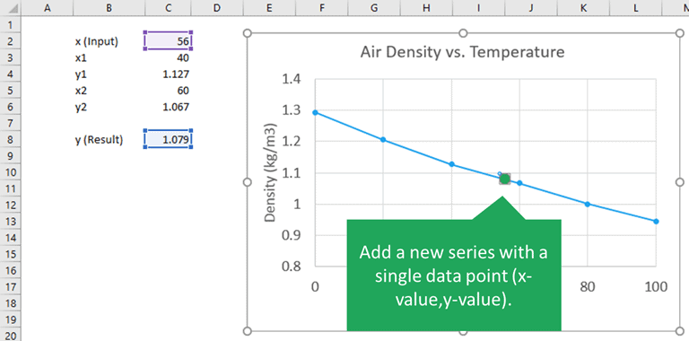
Add a DATA LABEL to ONE POINT on a chart in Excel - Excel Quick Help All the data points will be highlighted. Click again on the single point that you want to add a data label to. Right-click and select ' Add data label '. This is the key step! Right-click again on the data point itself (not the label) and select ' Format data label '. You can now configure the label as required — select the content of ...

How to Change Excel Chart Data Labels to Custom Values?

Add or remove data labels in a chart - support.microsoft.com On the Design tab, in the Chart Layouts group, click Add Chart Element, choose Data Labels, and then click None. Click a data label one time to select all data labels in a data series or two times to select just one data label that you want to delete, and then press DELETE. Right-click a data label, and then click Delete.

30 How To Add Label To Excel Chart - Labels Database 2020

How to hide zero data labels in chart in Excel? - ExtendOffice If you want to hide zero data labels in chart, please do as follow: 1. Right click at one of the data labels, and select Format Data Labels from the context menu. See screenshot: 2. In the Format Data Labels dialog, Click Number in left pane, then select Custom from the Category list box, and type #"" into the Format Code text box, and click Add button to add it to Type list box.

Share :