39 how to add different data labels in excel

5 New Charts to Visually Display Data in Excel 2019 - dummies Enter the labels and data. Put them in the order you want them to appear in the chart, from top to bottom. You can convert the range to a table to sort it more easily. Select the labels and data and then click Insert → Insert Waterfall, Funnel, Stock, Surface, or Radar Chart → Funnel. Format the chart as desired. 13 Essential Excel Functions for Data Entry Use TODAY () and NOW () with no arguments or characters in the parentheses. Just enter the following formula for the function you want, press Enter or Return, and each time you open your sheet, you'll be current. =TODAY () =NOW () Obtain Parts of a Text String: LEFT, RIGHT, and MID

How to Create and Customize a Treemap Chart in Microsoft Excel Select the data for the chart and head to the Insert tab. Click the "Hierarchy" drop-down arrow and select "Treemap." The chart will immediately display in your spreadsheet. And you can see how the rectangles are grouped within their categories along with how the sizes are determined.

How to add different data labels in excel

How to convert Word labels to excel spreadsheet - Microsoft Community 2345 Main Street Suite 200. Our Town, New York, 10111. or. John Smith. 1234 South St. My Town, NY 11110. I would like to move this date to a spreadsheet with the following columns. Title, Name, Business Name, Address, City State, zip. Some labels will not have a name or business name. How to Custom Format Cells in Excel (17 Examples) - ExcelDemy Custom. You can utilize the required format type under the custom option. To customize the format, go to the Home tab and select Format cell, as shown below. Note: you can open the Format Cells dialog box with the keyboard shortcut Ctrl + 1. How To Show Two Sets of Data on One Graph in Excel To do so, click and drag your mouse across all the data you want, including the names of the columns and rows. You can check that you selected the data by looking for the cells to be gray instead of white. 3. Click the "Insert" tab and then look at the "Recommended Charts" in the charts group

How to add different data labels in excel. Data labels on secondary axis position - Microsoft Tech Community Hi, I am wondering if there is a workaround (Mac)... When I make a horizontal bar graph with primary and secondary axes, I do not have a choice for label position to be "Outside End." Bars on the primary axis are stacked. But secondary axis bars are Clustered - Since the secondary axis is not stacked, why can't the labels be on the outside end ... How to add text or specific character to Excel cells - Ablebits To add certain text or character to the beginning of a cell, here's what you need to do: In the cell where you want to output the result, type the equals sign (=). Type the desired text inside the quotation marks. Type an ampersand symbol (&). Select the cell to which the text shall be added, and press Enter. How to mail merge and print labels from Excel - Ablebits When arranging the labels layout, place the cursor where you want to add a merge field. On the Mail Merge pane, click the More items… link. (Or click the Insert Merge Field button on the Mailings tab, in the Write & Insert Fields group). In the Insert Merge Field dialog, select the desired field and click Insert. Manage sensitivity labels in Office apps - Microsoft Purview ... If both of these conditions are met but you need to turn off the built-in labels in Windows Office apps, use the following Group Policy setting: Navigate to User Configuration/Administrative Templates/Microsoft Office 2016/Security Settings. Set Use the Sensitivity feature in Office to apply and view sensitivity labels to 0.

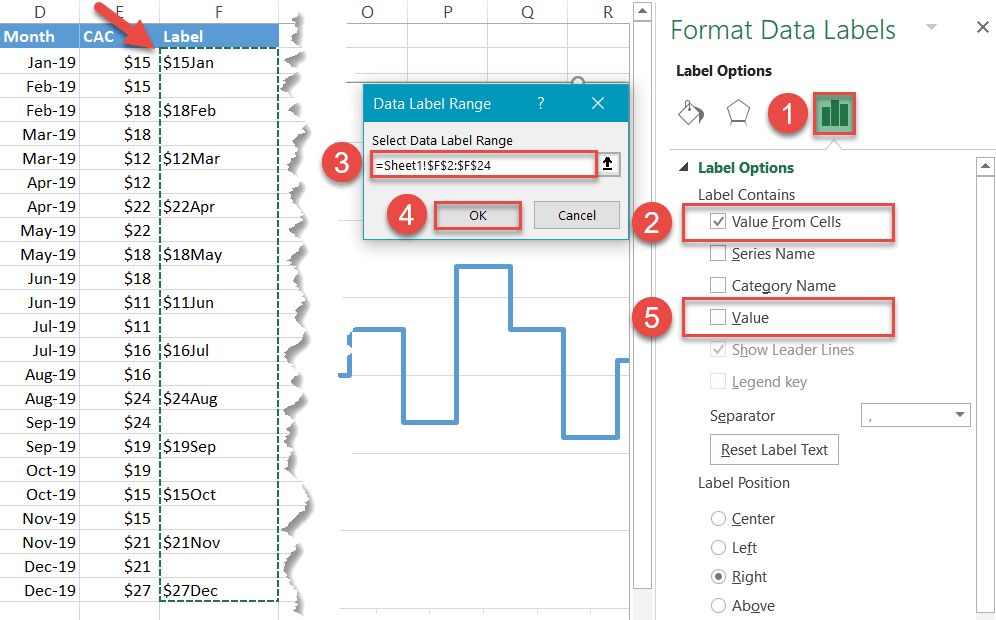
Chart.ApplyDataLabels method (Excel) | Microsoft Docs The type of data label to apply. True to show the legend key next to the point. The default value is False. True if the object automatically generates appropriate text based on content. For the Chart and Series objects, True if the series has leader lines. Pass a Boolean value to enable or disable the series name for the data label. › charts › dynamic-chart-dataCreate Dynamic Chart Data Labels with Slicers - Excel Campus Feb 10, 2016 · For now we will just add a cell that contains the index number, and point to the three metrics for each value in the CHOOSE formula. Eventually the slicer will control the index number. Step 5: Setup the Data Labels. The next step is to change the data labels so they display the values in the cells that contain our CHOOSE formulas. How To Create Labels In Excel - changeswinnipeg The data labels for the two lines are not, technically, "data labels" at all. Click "Ok" When You've Made Your Selection. Use the insert merge field button to select the fields in your excel file and add them to the label. The most common address label to use is a 5160 label size. Create the mail merge document in the microsoft word. How to Add Labels to Scatterplot Points in Excel - Statology Step 3: Add Labels to Points Next, click anywhere on the chart until a green plus (+) sign appears in the top right corner. Then click Data Labels, then click More Options… In the Format Data Labels window that appears on the right of the screen, uncheck the box next to Y Value and check the box next to Value From Cells.

Two-Level Axis Labels (Microsoft Excel) - ExcelTips (ribbon) Excel automatically recognizes that you have two rows being used for the X-axis labels, and formats the chart correctly. Since the X-axis labels appear beneath the chart data, the order of the label rows is reversed—exactly as mentioned at the first of this tip. (See Figure 1.) Figure 1. Two-level axis labels are created automatically by Excel. › make-labels-with-excel-4157653How to Print Labels from Excel - Lifewire Apr 05, 2022 · How to Print Labels From Excel . You can print mailing labels from Excel in a matter of minutes using the mail merge feature in Word. With neat columns and rows, sorting abilities, and data entry features, Excel might be the perfect application for entering and storing information like contact lists. How to trim and concatenate data in different cells? Thanks a lot. It is working, but it shouldn't result in last 2 > > "Furniture > Cabinets & Storage > >" If there is no data in the cell, it shouldn't add >. How to Use Excel Pivot Table Label Filters To change the Pivot Table option, and allow multiple filters, follow these steps: Right-click a cell in the pivot table, and click PivotTable Options. In the PivotTable Options dialog box, click the Totals & Filters tab. In the Filters section, add a check mark to 'Allow multiple filters per field.'. Click the OK button, to apply the setting ...

Excel charts: add title, customize chart axis, legend and data labels

mgconsulting.wordpress.com › 2013/12/09 › add-a-dataAdd a Data Callout Label to Charts in Excel 2013 Dec 09, 2013 · The new Data Callout Labels make it easier to show the details about the data series or its individual data points in a clear and easy to read format. How to Add a Data Callout Label. Click on the data series or chart. In the upper right corner, next to your chart, click the Chart Elements button (plus sign), and then click Data Labels.

Adding Data Labels to Your Chart (Microsoft Excel)

› documents › excelHow to add data labels from different column in an Excel chart? This method will introduce a solution to add all data labels from a different column in an Excel chart at the same time. Please do as follows: 1. Right click the data series in the chart, and select Add Data Labels > Add Data Labels from the context menu to add data labels. 2.

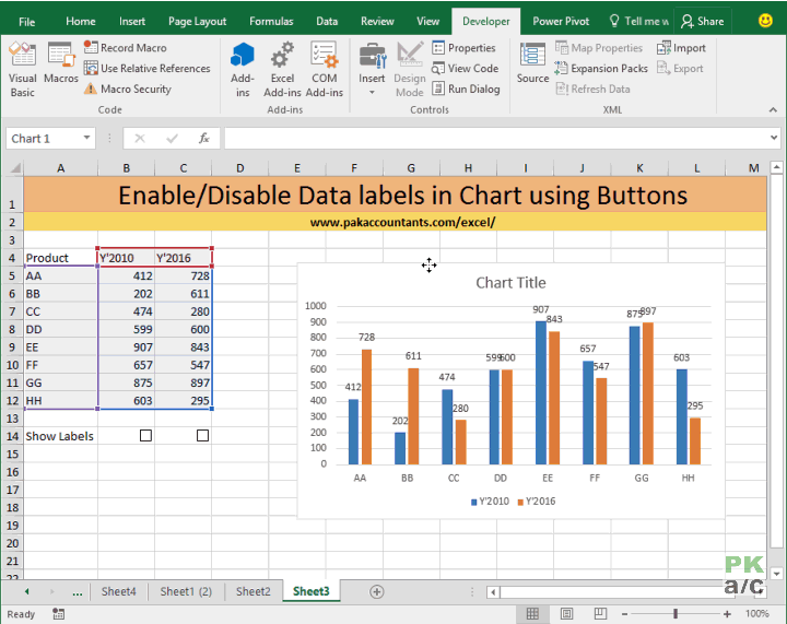
Enable or Disable Excel Data Labels at the click of a button - How To - PakAccountants.com

Excel: How to Create a Bubble Chart with Labels - Statology To add labels to the bubble chart, click anywhere on the chart and then click the green plus "+" sign in the top right corner. Then click the arrow next to Data Labels and then click More Options in the dropdown menu: In the panel that appears on the right side of the screen, check the box next to Value From Cells within the Label Options ...

Charting in Excel - Adding Data Labels - YouTube

How to Make and Print Labels from Excel with Mail Merge How to mail merge labels from Excel Open the "Mailings" tab of the Word ribbon and select "Start Mail Merge > Labels…". The mail merge feature will allow you to easily create labels and import data...

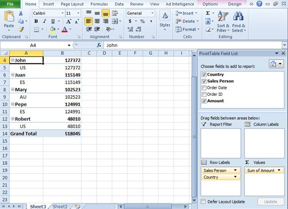
How to use Excel Pivot Tables

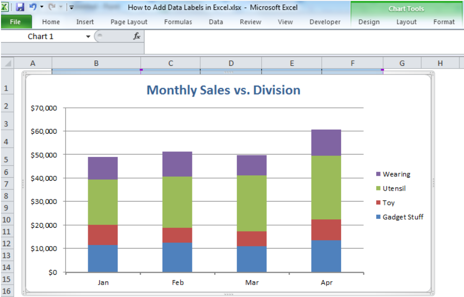
How to Create a Bar Chart in Excel with Multiple Bars? You can also add data labels. To add data labels, go to the Chart Design ribbon, and from the Add Chart Element, options select Add Data Labels. Adding data labels will add an extra flair to your graph. You can compare the score more easily and come to a conclusion faster. You can also choose a column chart that will give you a similar result.

How to Add Data Labels in Excel - Excelchat | Excelchat

How to Insert a Row in Excel 2013 (A Quick 4 Step Guide) How to Add a New Row in Excel 2013. Open your Excel file. Select the row number below where you want the new row. Click Home. Click the Insert arrow, then Insert Sheet Rows. Our article continues below with additional information on how to insert a row in Excel, including pictures of these steps. Have you ever meticulously entered a lot of data ...

How to Create a Step Chart in Excel - Automate Excel

How to match and extract different columns in excel How to match columns in excel. 1. Select the whole data set. Select Ctrl+A to highlight.. 2. And then click the Home tab. 3. Go to styles group and select conditional formatting.

Clustering

How To Add Data Labels In Excel » cahs July Right click the data series in the chart, and select add data labels > add data labels from the context menu to add data labels. Then click the chart elements, and check data labels, then you can click the arrow to choose an option about the data labels in the sub menu. Source: In excel 2013 or 2016.

How to create an Excel map chart

How to use cell values for excel chart labels - How to Right click the data series in the chart, and select Add Data Labels > Add Data Labels from the context menu to add data labels. 2. Click any data label to select all data labels, and then click the specified data label to select it only in the chart. 3.

Excel Chart Data Series, Data Points, and Data Labels

› excel › how-to-add-total-dataHow to Add Total Data Labels to the Excel Stacked Bar Chart Apr 03, 2013 · Step 4: Right click your new line chart and select “Add Data Labels” Step 5: Right click your new data labels and format them so that their label position is “Above”; also make the labels bold and increase the font size. Step 6: Right click the line, select “Format Data Series”; in the Line Color menu, select “No line” Step 7 ...

How to Add Data Labels in Excel - Excelchat | Excelchat

support.microsoft.com › en-us › officeAdd or remove data labels in a chart - support.microsoft.com Depending on what you want to highlight on a chart, you can add labels to one series, all the series (the whole chart), or one data point. Add data labels. You can add data labels to show the data point values from the Excel sheet in the chart. This step applies to Word for Mac only: On the View menu, click Print Layout.

Enable or Disable Excel Data Labels at the click of a button - How To - PakAccountants.com

How to Create Excel Drop Down List with Color (2 Ways) Creating Drop Down List. To begin with, select the cell or cell range to apply Data Validation. ⏩ I selected the cell range E4:E12. Open the Data tab >> from Data Tools >> select Data Validation. A dialog box will pop up. From validation criteria select the option you want to use in Allow. ⏩ I selected List.

Missing Values - SAS Tutorials - LibGuides at Kent State University

How to Use Excel's Descriptive Statistics for Data Analysis How to Add Data Analysis to Excel Before you can use the Data Statistics tool, you need to install Excel's Data Analysis ToolPak. To do this, click on File > Properties > Add-Ins. At the bottom, where it says Manage, click on Go... In the new window that pops up, make sure that you have the Analysis ToolPak checked.

Add or remove data labels in a chart - Office Support

How To Add a Target Line in Excel (Using Two Different Methods) Open Excel on your device. In order to add a target line in Excel, first, open the program on your device. Either click on the Excel icon or type it into your application search bar. Once you open Excel, you can either create a new spreadsheet or edit an existing one. 2.

How to Create Multi-Category Chart in Excel - Excel Board

chandoo.org › wp › change-data-labels-in-chartsHow to Change Excel Chart Data Labels to Custom Values? May 05, 2010 · First add data labels to the chart (Layout Ribbon > Data Labels) Define the new data label values in a bunch of cells, like this: Now, click on any data label. This will select “all” data labels. Now click once again. At this point excel will select only one data label.

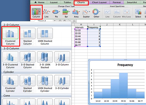
Create a Histogram Graph in Excel

How To Show Two Sets of Data on One Graph in Excel To do so, click and drag your mouse across all the data you want, including the names of the columns and rows. You can check that you selected the data by looking for the cells to be gray instead of white. 3. Click the "Insert" tab and then look at the "Recommended Charts" in the charts group

Share :